Projecting The MLB Season: Creating a Model
Major League Baseball has mandated a 60 game season, which will cause changes in the playoffs. Baseball is the proverbial marathon where one game doesn’t mean as much given the amount of games played. Over a 162 game season, the cream rises to the top. For instance, the Los Angeles Dodgers are the projected best team in baseball. They’ve won seven straight division titles, have won over 100 games in two of the last three years, and have lost two of the last three World Series. The club’s farm system ranks, post 2020 MLB Draft, third per FanGraphs, expected to sign the seventh best International player, and they invest heavily in player development. Their farm is great, player development is great, have had a great run of success, and are projected to win 97 by FanGraphs and 103 by Baseball Prospectus.
Even with all that success and talent, both in the farm and on the Major League roster, the Dodgers in an 81 game season see their playoff odds fall by 27.3 percentage points. Given the more variance involved, the better teams are worse off, but that holds even more true in a 60 game season. Eno Sarris, of The Athletic, looked at what the level of games means in describing a season. He describes the level at different proposals, 48 and 89, but looking at his When Do We Know If a Team is Good graph, a team’s winning percentage at 60 games explains about 70 percent of a their end of season record. There’s more variance involved and worse teams will look better through 60 games.
But given baseball is back, I wanted to create a basic model that will project how many games each team will win given their schedule. To start with, I looked at the original 2020 schedule, where the season would be 162 games long. I followed along with the steps in Analyzing Baseball with R, which uses a Bradley-Terry model to predict the win probability of each game. I obtained the schedule from retrosheet, but I needed a proxy for talent to be used in the model. I decided to use the over/under consensus from Betting Pros and translated it to talent by using [over – 81]/81 to get a mean talent at 0. The home team wins around 55 percent of the time (about 54 percent per this Baseball Prospectus article in 2009), so we have to adjust for the home field advantage. To control for some teams being better, I averaged the home field advantage to be 55 percent; if the visiting team had a higher talent level than the home team, the visiting team’s talent level was reduced by 0.025 and the home team’s talent level was increased by 0.025. If the home team had the higher talent level, the visiting team’s talent level was reduced by 0.075 and the home team’s talent level increased by 0.075.
This leads to the following results (the table is scrollable), showing the lower bound, average, and upper bound of wins:
| Team | Lower Bound | Average Wins | Upper Bound |
|---|---|---|---|
| Dodgers | 82 | 95 | 107 |
| Yankees | 82 | 94 | 106 |
| Astros | 79 | 91 | 103 |
| Twins | 78 | 90 | 102 |
| Rays | 76 | 89 | 101 |
| Braves | 75 | 88 | 100 |
| Athletics | 75 | 87 | 99 |
| Nationals | 74 | 86 | 98 |
| Indians | 73 | 85 | 97 |
| Cardinals | 72 | 84 | 97 |
| Cubs | 72 | 84 | 96 |
| Mets | 71 | 84 | 96 |
| White Sox | 71 | 84 | 96 |
| Angels | 70 | 83 | 95 |
| Phillies | 70 | 83 | 95 |
| Red Sox | 71 | 83 | 95 |
| Brewers | 69 | 82 | 94 |
| Diamondbacks | 69 | 82 | 94 |
| Reds | 70 | 82 | 95 |
| Padres | 69 | 81 | 94 |
| Rangers | 66 | 78 | 91 |
| Blue Jays | 64 | 76 | 89 |
| Rockies | 62 | 74 | 87 |
| Giants | 60 | 72 | 84 |
| Pirates | 60 | 72 | 84 |
| Royals | 59 | 71 | 84 |
| Mariners | 58 | 70 | 83 |
| Marlins | 56 | 68 | 81 |
| Tigers | 54 | 66 | 78 |
| Orioles | 53 | 65 | 77 |
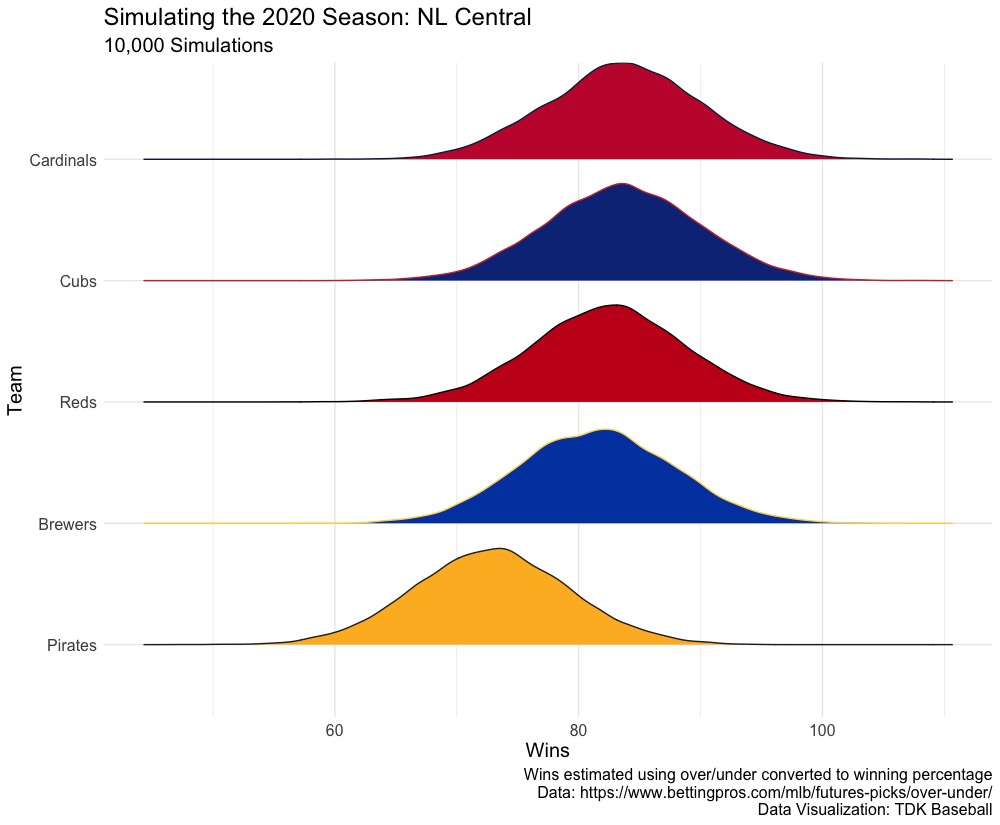
One way this helps is visualizing the talent in a division. For example, here is the National League Central:
| Team | Lower Bound | Average Wins | Upper Bound |
|---|---|---|---|
| Cardinals | 71 | 84 | 96 |
| Cubs | 71 | 84 | 96 |
| Reds | 70 | 82 | 95 |
| Brewers | 69 | 82 | 94 |
| Pirates | 60 | 73 | 85 |
Considering the over/under bets have the Brewers, Reds, Cardinals, and Cubs between 83 and 86 games, the NL Central looks to be competitive, with the Pirates lacking behind. The distribution of the simulations looks:

It’s a simple simulation model, but here’s how this model, the consensus over/under, FanGraphs, and PECOTA projections:
| Simple Simulation | Consensus Over/Under | PECOTA | FanGraphs | |
| Simple Simulation | 1.00 | 0.99 | 0.93 | 0.97 |
| Consensus Over/Under | 0.99 | 1.00 | 0.93 | 0.97 |
| PECOTA | 0.93 | 0.93 | 1.00 | 0.96 |
| FanGraphs | 0.97 | 0.97 | 0.96 | 1.00 |
It’s no surprise that the simple simulation correlates nearly perfectly with the over/under as the model is based on the over/under. But it’s highly correlated with PECOTA (0.93) and FanGraphs (0.97). The market is generally correct, given the wisdom of the crowds. So let’s use the simulation to project the probability of winning the division per 10,000 simulations. Here’s the NL Central, again, for example:
| Team | Division Odds |
|---|---|
| Cardinals | 0.2856 |
| Cubs | 0.2791 |
| Reds | 0.2256 |
| Brewers | 0.1890 |
| Pirates | 0.0207 |
In 28.56 percent of the simulations, the Cardinals won the division, but that was only six points higher than the third place Cincinnati Reds. The division will be a close battle, unlike the NL West (Dodgers at 81.5 percent), AL West (Yankees at 66.2 percent), AL Central (Twins at 55.8 percent and Indians at 24 percent, a two team race with a heavy favorite), and AL West (Astros at 54.7 percent and Athletics at 27.5 percent, another two team race with a heavy favorite). Here’s how the simple simulation, PECOTA, and FanGraphs division odds correlate:
| Simple Simulation | PECOTA | FanGraphs | |
| Simple Simulation | 1.00 | 0.90 | 0.96 |
| PECOTA | 0.90 | 1.00 | 0.93 |
| FanGraphs | 0.96 | 0.93 | 1.00 |
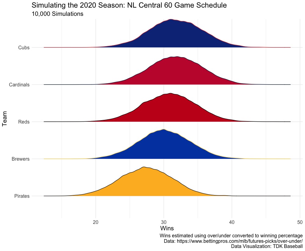
We can use this simple model as a talent level indicator to show the level of variance and division odds changes in a 60 game schedule, again using the NL Central. We know that the schedule will be 60 games with 40 against the division and 20 against the interleague division, with six being the natural rival. This is how the NL Central will look like against the AL Central, with assumptions in the two three game sets and the two four game sets:
| Natural Rival | Three Game Sets | Four Game Sets | |
|---|---|---|---|
| Cardinals | Royals | Indians, Tigers | Twins, White Sox |
| Cubs | White Sox | Indians, Twins | Tigers, Royals |
| Reds | Indians | Twins, Royals | White Sox, Tigers |
| Brewers | Twins | Indians, Tigers | Royals, White Sox |
| Pirates | Tigers | Royals, White Sox | Indians, Twins |
That schedule is just a mock and no way is a real schedule (it has to balance out at each team having 30 home games and I believe the above makes it unlikely to do so), but based on it, we get the following distribution of wins and playoff odds:

| Team | Lower Bound | Average Wins | Upper Bound | Division Odds |
|---|---|---|---|---|
| Cubs | 24 | 32 | 39 | 0.2934 |
| Cardinals | 24 | 32 | 39 | 0.2848 |
| Reds | 23 | 31 | 38 | 0.2106 |
| Brewers | 23 | 30 | 38 | 0.1593 |
| Pirates | 20 | 27 | 35 | 0.0519 |
In the 60 game season on the mock schedule, the teams are even closer together, with the Pirates seeing their division odds increase from 2.07 percent to 5.19 percent, and the Cubs even overtook the Cardinals. When the actual schedules get released, I will run all 30 teams to get the true division odds and true estimated wins.
Where this model falls short is that it’s just based on the over/under lines. A better model would use their team run projections, controlling for each games expected starter, injury risk over a season, and player transactions, either internally or externally. This simple model using the over/under can help in setting the prior with a bayesian approach. After each game, the model can be updated with the likelihood their record reflects their end of season record and transitioning everything to a run differential model, where the prior is using the translated over/under to translated run differential.
Leave a Reply