Evaluating MLB Hitters: Creating a Model

Statcast, through the use of Trackman and soon to be Hawkeye, has provided data on exit velocities, launch angles, and other varies inputs. This allowed Dr. Jim Albert, of Bowling Green State, to creating a model to estimate the probability of a batted ball being a hit based on the exit velocity, launch angle, and the calculated spray angle using the process laid out by Bill Petti. We know that slugging percentage varies based on the launch angle and exit velocity of any batted ball, but where on the field that ball is hit is also important to know; a ball that is pulled is more likely to be a home run than a ball hit to centerfield. That is something that’s been intuitive and a common understanding throughout the game of baseball, especially as the depth of fences down the foul lines are shorter than that of dead center. These measurements allow for an estimated batter model to be created, such as estimated wOBA; for the concepts of the model created for this website, I’ll be using the methods described above from Dr. Albert. All the data was downloaded using Baseball Savant’s website and analyzed in the statistical software R.

***

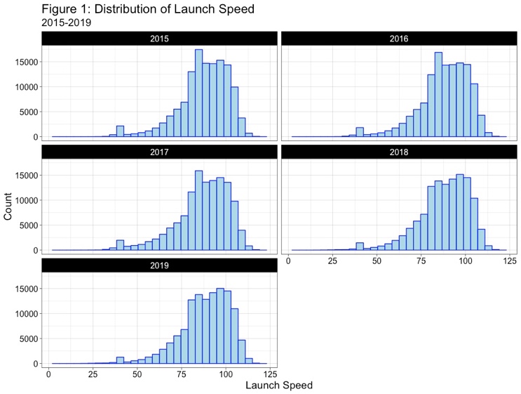
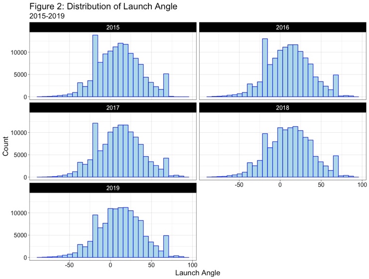
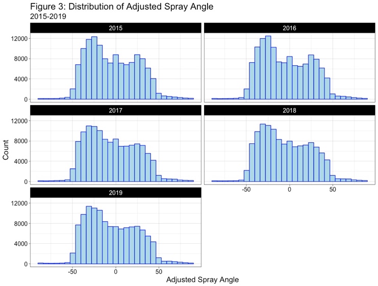
Understanding the data is important. Looking at the launch speed (exit velocity), launch angle, and the adjusted spray angle, we can see that the average ball is hit about 1.0 mph harder in 2019 than 2015, is hit at angle that is about 2.0º higher than a ball in 2015, and is pulled 0.7º more. The table below displays the mean values with the standard deviation underneath in parentheses:

	Launch Speed	Launch Angle	Adjusted Spray
2015	87.3 mph (14.2 mph)	10.1º (26.9º)	-3.9º (28.5º)
2016	87.7 mph (14.1 mph)	10.8º (27.3º)	-4.2º (28.7º)
2017	86.7 mph (15.1 mph)	11.1º (27.6º)	-4.7º (28.6º)
2018	87.7 mph (14.3 mph)	11.7º (27.6º)	-4.5º (28.7º)
2019	88.1 mph (14.2 mph)	12.2º (27.4º)	-4.6º (28.6º)

Given the numbers not the easiest to visualize, the three figures below show the distribution of batted balls by year for the three variables listed above:

While Dr. Albert used just the three variables of launch speed, launch angle, and adjusted spray angle, the year will be included as a fourth variable given the changing of the run environment and the differences of the baseball. Dr. Albert used a generalized additive model (GAM), where E(hit | launch speed, launch angle, adjusted spray angle, year) = β +s1(launch speed) + s2(launch angle) + s3 (adjusted spray angle) + s4(year). By taking the inverse logit, P(batted ball = hit) = (e^hit)/(1+e^hit), where hit is the model above. Building off Dr. Albert’s work, we can replace hit with the four hit types – single, double, triple, and home run – and define the variables such that the event = 1, otherwise = 0. For example, double = 1 if batted ball is a double, 0 otherwise. We then replace hit in Dr. Albert’s GAM with the batted ball type and the probability that the batted ball is one of those hit outcomes is estimated.

By summing the results by year, you get the estimated batting outcomes of balls in play for each player. Since some parks are more hitter friendly, Coors Field, and some more pitcher friendly, Comerica Park, it’s important to park neutralize the data, allowing for all players to be compared on the same scale. The park factor is then the estimated results/actual results, creating a park factor for each individual park each season. For instance, if there were 105 singles in a season at PNC Park but an estimated 98, the park factor singles in that season would be 0.93. Using these park factors, each component was then park neutralized, by using the player’s home stadium park factor. This can help in another way: how many more or less home runs would we expect a newly acquired player to hit in our stadium?

Using the seasonal numbers for at bats, walks, hit by pitches, and sac flies, an estimated batting average, estimated slugging, estimated ISO, estimated BABIP, and estimated wOBA can be created, which I define as est_[stat]. Calculating the league est_wOBA, as seen in the table below, helps in creating an estimated runs added measurement.

	League est_wOBA
2015	.314
2016	.318
2017	.320
2018	.313
2019	.319

Estimated runs is just wRAA but with the est_wOBA for player and league in place of wOBA. The top players by the estimated runs model are:

Year	Player	estimated runs	runs
2016	David Ortiz	75.93	52.2
2015	Joey Votto	72.22	63.1
2017	Charlie Blackmon	71.58	57.2
2015	Chris Davis	69.62	40.9
2017	Nolan Arenado	67.17	42.6

With about 10 runs equaling a win, David Ortiz provided the Boston Red Sox with about 7.6 wins just from his bat. Joey Votto provided the Cincinnati Reds with 7.2 wins with just his bat. These numbers don’t account for position, defense, or base running, and as such will be presented as just runs on the site.

***

Baseball Prospectus has laid out principles for baseball analysis, including three important performance measures: Descriptive, Reliability, and Predictability. When looking at the expected stats from Statcast, Jonathan Judge ran 100,000 bootstrapped re-samples to calculate the mean correlation and their errors, a similar method to what he did with catcher framing data. By adapting their code to fit our variables, we can run their tests in the same manner to check for those three measurements.

The first test I looked at was wOBA compared to est_wOBA, where the mean correlation is listed with the error in parentheses below:

	Descriptive (This year’s wOBA)	Reliability (Next year’s metric)	Predictability (Next year’s wOBA)
wOBA	1.000 (0.000)	0.485 (0.023)	0.485 (0.023)
est_wOBA	0.861 (0.009)	0.623 (0.023)	0.496 (0.023)

The estimated wOBA describes wOBA pretty well, correlated at 0.861, correlating with the previous results. The model is also more reliable than wOBA in year t+1, correlating with itself in year t+1 at 0.623 compared to wOBA’s correlation of just 0.485. The lower bound for the reliability of the estimated wOBA is 0.600 and the upper bound for wOBA is 0.508. Since the confidence intervals don’t overlap, the estimated wOBA model is more reliable year-over-year than wOBA. In predicting next year’s wOBA (wOBA in year t+1), the estimated wOBA model comes out on top compared to wOBA, but there is overlap with the margin of errors, so we can’t confidently claim that this estimated wOBA model is better at predicting wOBA in year t+1.

The final test was looking at batting average using batting average, babip, and the estimated batting average and estimated babip models. The table is the same as above:

	Descriptive (This year’s ba)	Reliability (Next year’s metric)	Predictability (Next year’s ba)
ba	1.000 (0.000)	0.473 (0.028)	0.473 (0.028)
babip	0.747 (0.014)	0.372 (0.031)	0.284 (0.032)
est_ba	0.789 (0.013)	0.575 (0.026)	0.447 (0.030)
est_babip	0.554 (0.020)	0.399 (0.030)	0.242 (0.034)

In describing this year’s batting average, babip and the estimated batting average do well, with the estimated batting average doing a better job at describing the previous results. The estimated babip model does poorly and is not as correlated with batting average as compared to the other two. The estimated batting average model is the most stable followed by batting average, with estimated bapip having the edge over babip, though that comes with overlap with the errors. In terms of predicting year t+1 batting average, batting average in year t is the best, followed by the estimated batting average model, where there is some overlap, but the edge goes to batting average. Babip and the estimated babip model fall in the final two spots, with the estimated babip model finishing in last at both describing batting average in year t and predicting batting average in year t+1.

***

This estimated batting model originally started off as a school project for an economics elective during the winter/spring of 2019, estimating only wOBA and run values by building off the work that Dr. Jim Albert has produced on his website. In essence, this is his general model that was adapted to model each type of hit and translate into a wOBA model where a park factor was calculated in order to calculate the adjustments. Since that elective was taken a year and a half ago, this project has evolved into adding the estimated batting average, slugging percentage, isolated power, and babip numbers. It has since been updated to include these numbers for splits against right handed and left handed pitching.

These numbers can be found on the Batting Stats tab on the website. There are three tabs with the Batting Stats for numbers by team (for example, Edwin Encarnacion’s 2019 numbers with the Seattle Mariners and the New York Yankees), overall season numbers (Encarnacion’s 2019 season), and by splits (Encarnacion’s vs right and left handed pitching). The column visibility tab will hide and unhide columns in the table as the total amount of columns makes the table too wide for viewing. More information is presented in the Batting Stats tab.